"What is X?" - Modeling the Meltdown

"What is X?" - Modeling the 2008-2009 Financial Systems Meltdown

We're about to start a detailed walkthrough of applying a "simple" statistical thermodynamic model to the Wall Street players in the 2007-2009 timeframe. The two kinds of information that I'll be joining together for this will be a description of Wall Street dynamics, based largely on Chasing Goldman Sachs (see previous blogposts for link), and the two-state Ising thermodynamic model that I've been presenting over the past several posts.

The model first. The first and most important thing that we have to determine when we're applying a model is: What are the key variables and parameters, and what do they mean? To do this, we need to have an a priori understanding of the model itself - how it behaves, what it could possibly provide for us in terms of understanding (and even predicting) a situation.

The model that I've been taking us through is based on modeling a system of a fairly large number of "units," where each "unit" can be either "on" or "off"; or "active" or "inactive," depending on our point of view. The important thing here is: If we want to use this model, we're having to make the very dramatic simplification that all the "units" that we're modeling are in one of only two possible states. This is an extreme simplification. The value of making this simplification will show up only if the model, at the end of making all the parameter assignment and turning the "model crank," we get some sort of interesting answer. (This is kind of like reading a mystery novel, we don't know how it will turn out until the end.)

In our case, the simplification that we're going to make is this:
1) We will make the "units" be all the active players on Wall Street that could possibly engage in some sort of highly leveraged buy-out or other fairly extreme (leveraged, risky) undertaking. This includes both buy-side and sell-side. It includes the banks, the hedge funds, and - essentially - all the players. The only question is: Were they involved in a "risky" (or "highly leveraged") transaction or not?
2) Then, x - the only real "variable" in our system - represents the fraction of the total number of "units" (banks, hedge funds, whatever) that were involved in such transactions at a given time.

We start our walkthrough with being at Point 1 of yesterday's blog, in Region A. Region A is the area where there is only one free energy minimum. That means, there is only one "stable state." For Region A, this minimum occurs for a relatively low value of x, as is shown in the following Figure 1.

We can see that in this Figure 1 (characteristic for all of Region A), the value of x giving the free energy minimum is about at x=0.1.

So this doesn't mean that no banks, hedge funds, etc. were engaged in risky deals - just that a very small fraction of the overall number of banks, hedge funds, etc. were so involved. Goldman Sachs, for example, took some early strategic steps that were risky (highly leveraged), but it distributed its risk by taking on diverse plays.

If we're going to apply this model, we now need to identify the meaning of the two parameters involved; e1 and a=e2/e1.

When we look at the phase space diagrams of previous posts, we see that there are two parameters. The one across the top (ranging from 1.5 to 8.5) is e1. (I'm using a simplified notation here compared to the Greek letters and subscripting in the equations themselves.) e1 represents an "activation energy," or the "energy cost" (enthalpy per unit) of having a unit in an active state.

Let's have a quick review of basic thermodynamic principles. A system is "at equilibrium" when the free energy at a minimum. (In the Figure 1 for this post, this occurs when x is about 0.1.) Free energy is enthalpy minus (a constant times) entropy. (We work with the "reduced" free energy for all of our discussions, where constants and other terms have been divided out, subtracted out, or otherwise normalized; so all future references to enthalpy will really mean a "reduced" enthalpy where various constants have been worked to give a simpler, cleaner equation.)

As per our first equation, several blogposts ago, we really have two enthalpy terms; one is an enthalpy-per-active unit (linear in x), and the other is an interaction energy term, which is an "interaction energy" times x-squared.

The enthalpy-per-active-unit is e1.

If we're going to make this model work, we need to figure out what this means.

Suppose that we took our basic free energy equation, and pretended that there was no enthalpy at all; there was no extra "energy" put into the system when the various units were "on" or "off." Then the free energy would be at a minimum when the entropy was at a maximum, and this occurs when x=0.5. (The entropy equation here is symmetric; entropy = x(ln(x)+(1-x)ln(1-x).

What happens when we introduce the enthalpy terms is that we "skew" the free energy minimum to one side or another. Region A corresponds to the area where the interaction energy is low, so for the moment, let's pretend that it doesn't exist. We'll focus on the physical meaning of the parameter e1. It is to be something that will shift the free energy minimum to the left, or make the value of x that produces a free energy minimum to be smaller. (In Figure 1, the free energy is at a minimum when x=0.1 instead of 0.5.)

The enthalpy-per-unit term, e1, associated with Region A (and in fact all of Figure 1) is a positive term. It means that there is an "energy cost" to having a unit in an active state.

We're going to interpret this cost as risk. We will say that e1 models the risk for a unit (a bank, a hedge fund, etc.) to be involved in a very leveraged transaction. The risk can be small (e1=2) or large (e1=7). Either way, we get a single minimum if there is no "interaction" energy; this minimum is for a low value of x, meaning that relatively few units are "on" or are involved in risky transactions.

Now we come to the "crux of the biscuit." What does the other parameter, a, mean? This is our interaction-energy term; it multiplies x-squared. We get the "interesting behavior" in Region D (the middle, pink region of the phase space diagram of yesterday's post). And in order to get the system to move from what we'd think of as a "logical, sane" equilibrium state - one in which relatively few units are involved in risky transactions - to the equilibrium state of Regions F or G (where most of the units are "on") - something has to happen. Something has to "force" more units to take on more "risk."

This "something" has to do with how the units interact with each other.

What would this mean in Wall Street social and political dynamics? How about peer pressure? Think about it. Interaction-energy = peer pressure. This is how banks and other institutions - who knew that what they were doing was not only risky, but downright foolhardy - were moving into these highly leveraged situations.

In terms of Figure 1 of the previous post, the whole system of Wall Street financial institutions were going from Point 1 to Point 2 to Point 3. By the time the system was in Point 3, almost all units were involved in risky transactions (I'll show the free energy diagram in the next posting), and the "free energy minimum" was VERY deep. And there was no "alternative." There was only a single free energy minimum. In other words, the whole system was trapped in a very risky situation.

Tracing the Financial Meltdown of 2008-9

Tracing the 2008-2009 Financial Meltdown Through a Metastable Phase Space

We can trace a path through the phase space shown in Figure 1 that shows the same kind of behavior as the financial world went through during the 2008-2009 meltdown.

Figure 1 shows a "path" going from a low-active state to a high-active state (3) back to low-active state (7) again. (To be continued)

Modeling a Financial Meltdown Using Metastable State Phase Transitions

Modeling the 2008-2009 Financial Meltdown Using Metastable State Phase Transitions

Now that we've weathered the crisis of 2008-2009, we can prudently ask ourselves: "What are the warning signs of imminent meltdown? How can we predict - and act prior to - a major market collapse?"

This post continues the theme begun in the previous post, of playing with a not-quite Gedanken experiment; looking for a useful model that explains what happened with the U.S. financial system at the end of 2008 and early 2009.

The important contribution of this post is that it presents a graphical representation of a model (free energy from statistical thermodynamics) that allows a system to be in a metastable state. This would characterize the overall banking/private equity/leveraged buy-out industry in 2008, just prior to the meltdown.

The following Figure 1 shows a "reduced" (parameter-normalized) free energy F* as a function of x, where x can range from 0 to 1. (For the free energy equation, and discussion thereof, see Phase Spaces: Mapping Complex Systems.

Figure 1: Set of five free energy graphs; F* versus x, where F* is the "reduced" (re-parameterized) free energy, and x represents the fraction of units in the system in an "on" or "activated" state. The five different graphs are obtained for different combinations of enthalpy parameters (to be discussed in a following post). The topmost graph refers to Region A (see following Figure 2), in which only a single free energy minimum exists, and is for a low value of x. The middle three graphs are for parameter values taken from Region D of Figure 2; these allow for double minima to appear. That means that a system can be in either a low-x or high-x state. (Relatively few activated units, or almost all units active.) The lowest graph corresponds to Region F, for which only a single free energy minimum exists, but this time with a high value of x (most units are "active" or "on.")

For reference, Figure 2 reproduces the phase space for different types of free energy graphs, originally presented and discussed in Phase Spaces: Mapping Complex Systems. Table 1, which summarizes the characteristics of these different regions, was also presented in that post.

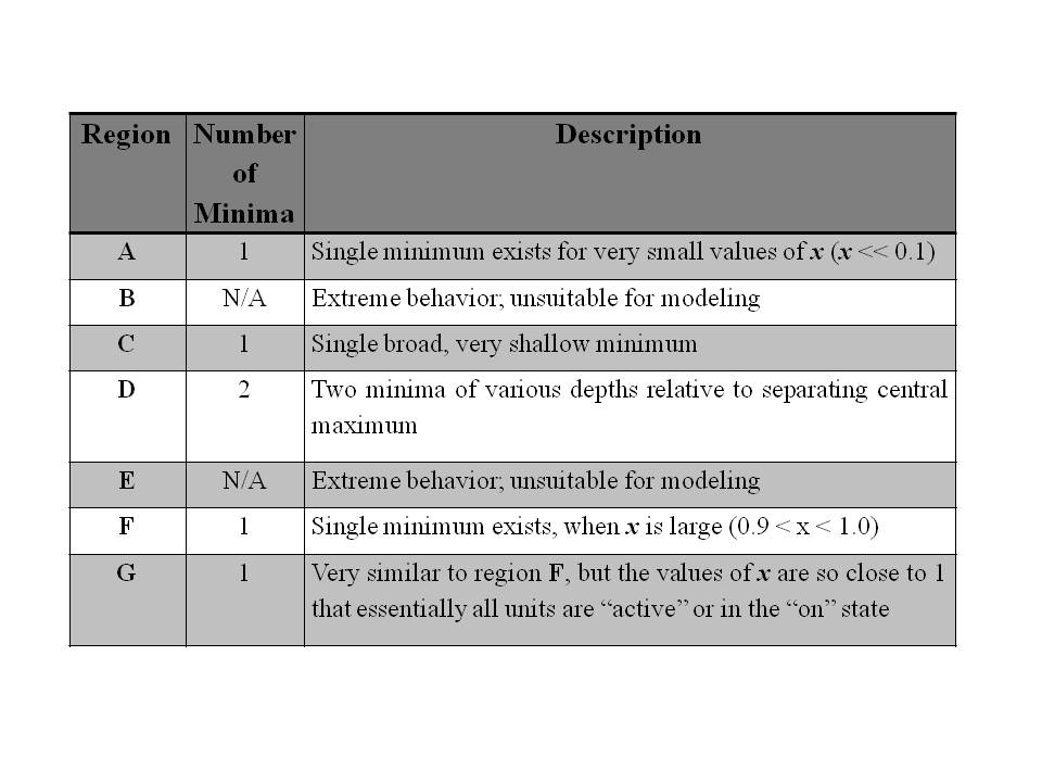
Figure 2 shows a phase space of seven distinct regions, labeled A-G. These regions are characterized in the following Table 1.

Table 1: The regions identified as A-G in the preceding Figure 2 are characterized in terms of number of (reduced) free energy minima, and whether these minima correspond to low, high, or both low and high values of x.

The important thing about this Figure 2 phase space diagram, and the distinct regions within it, is that it shows how a phase transition could happen between two very different states in a system; one where x is high (most units are in a very active or "on" state x=> 1), and another in which x is low (most units are in an inactive or "off" state, x=>0).

To see this possibility, please go to the discussion presented in Phase Spaces: Mapping Complex Systems.

The important previous blogpost references for this post are:
1) Some statistical thermodynamics theory (basic Ising spin-glass theory, with interacting bistate units), established in Phase Spaces: Mapping Complex Systems, and
2) Chasing Goldman Sachs, by Suzanne McGee, discussed in the previous post, Modeling a Financial Nonlinear Phase Transition.

As a starting point, I am using the basic Ising model development outlined by Goldenfeld in his Lectures on Phase Transitions and the Renormalization Group, as well as a paper by Pelizzola that describes the Cluster Variation Method (CVM) in relation with graph theory.



The core idea that I will use for this discussion is that at the time of the meltdown, the various "key players" were in a highly metastable state.

In nature, it is common for systems to "tend towards equilibrium." This means that they seek a balance between enthalpy (the energy associated with each component of the system) and entropy (the tendency of a system to move towards greatest possible dispersal among all possible energy and association configurations).

A systems's free energy (F) represents the dynamic tension between the two factors of minimizing overall system enthalpy and maximizing overall entropy. When free energy is at a minimum, we say that a system is in equilibrium.

Often, in nature, when conditions change, a system will adjust its composition to keep its free energy at a minimum (to stay in equilibrium). However, not all systems can respond adequately, even when the conditions under which they are operating change substantially. Instead, they sometimes go into a metastable state; a state which is locally a free energy minimum, but not the true, overall free energy minimum. However, the system will persist in this metastable state until conditions change so much that the little, local free energy "well" which it was inhabiting disappears completely. Then, it has no recourse. It will slide into its true "minimal free energy state," that is, it will move into equilibrium.

Modeling a Financial Nonlinear Phase Transition

A disclaimer. Before you (or I) go any further with this, an upfront and blanket disclaimer.

This is not a real, true, serious modeling effort.

It is not even a true gedanken-experiment (German for "mental experiment," or mental walk-through.)

If anything, this is a little warm-up exercise. An attempt to stretch and flex some "modeling muscles" that have not been used for a couple of years. (And in good cause, I might add - I've just completed a book, see Unveiling: The Inner Journey.

Writing that book fulfilled a private passion that had taken sixteen years to come to completion; the last two years were nearly full-time spent on writing and rewriting, editing and re-editing, proofing and re-proofing, plus a great deal of reference-checking, index-building, and related activities. But even the cover art is now done (or it will be soon), and I am deeply drawn back to another passion - that of modeling complex, nonlinear systems. Especially systems that tend to go "boom!"

Such is the case with the financial meltdown of 2008-2009. I'm listening (once again) to Suzanne McGee's Chasing Goldman Sachs. I stopped the CD somewhere around Chapter 4, when she was describing how highly-leveraged buyouts climbed to an increasing crescendo. We knew, of course, that the collapse was coming. Could this be described as a phase transition?

Modeling Financial Meltdown as a Phase Transition

The financial system described by McGee in Chasing Goldman Sachs
has an increasing number of institutions - both private-equity and hedge funds on the one side, and companies being purchased on the other side, together with the institutions that enable these transactions - involved in buyouts. The frequency became so great, along with the number of repeated sales of certain companies, that it became clear that this was no buy-and-reformulate strategy. As McGee plainly states, "These were flips." And the increase in activity was reaching frenetic proportions.

So - again firmly caveating; this is simply a warm-up exercise; this is "play" - not a real serious attempt at modeling - could we model this as a phase transition?

If so, the first and most important question is the one that I posited in a recent posting, namely Modeling Nonlinear Systems: What is x?

That will be the subject of the next posting.

Rebooting - and Next Stage

Yesterday met with graphics artist/multimedia specialist, the gorgeous Katerina Merezhinsky, who is completing the cover art for my soon-to-be-released latest book, Unveiling: The Inner Journey. What a big transition point! One book will be available shortly, and I'm already feeling drawn to starting the next - this time going back to my earlier interests in nonequilibrium systems as a means for modeling complex and emergent behaviors.

My new motto is "Physics first," and am starting the day with reviewing Pelizzola's excellent article on
Cluster Variation Method in Statistical Physics and Probabilistic Graphical
Meodels,. (I've just created a link to this article from my Nonlinear Forecasting Resources webpage.) This paper is important because it overviews the Cluster Variation Method (CVM) in context of its relation with other approaches, specifically with belief propagation networks and graph theory. The connection between these two is exciting, because CVM is a powerful computational method, with roots in statistical thermodynamics, and graph theory - as an organizing principle - links many domains of interest and potential applications.

Modeling Nonlinear Phenomena

Modeling Nonlinear Phenomena - What is "X"?

Many of us grew up hating word problems in algebra. (Some of us found them interesting, sometimes easy, and sometimes fun. We were the minority.)

For most of us, even if we understood the mathematical formulas, there was a big "gap" in our understanding and intuition when it came to applying the formulas to some real-world situation. In the problem, we'd be given a set of statements, and then told to find "something." We were supposed to turn these "starting statements" into mathematical statements of what we knew. That is, we had to say, "Let X = (something)." "X" could be the speed of a car, the distance between two cities; it could be anything among the set of known facts. Then we had to make similar "mathematical statements" about other information that was given to us. And then, we were to say, "Now I want to find Y, my 'unknown.'"

All very well and good, when we're doing algebra, and the answers are in the back of the book. (Or at least the teacher will review and correct our work.) And just slightly more difficult when we are in the "real world."

Years ago (many more years than I care to acknowledge), I made a crucial "life-decision." I knew that I was interested in the capabilities of our minds and our brains. I knew that this area was getting more and more complex, with each passing year. And, given my gift for mathematics and abstract thinking, I decided that I wanted to learn how to make mathematical models of complex situations.

I didn't know exactly how I would use such an ability, I just knew that I needed to learn the fundamentals.

So I spent the next several years happily studying quantum mechanics and statistical thermodynamics, both of which were mathematically elegant and satisfying at the soul-level. Kind of like learning mathematical analogues to poetry.

I've had many opportunities to rejoice that I took on such a disciplined formal approach when I was younger, because now that knowledge serves me well. Even more, the discipline of the approach - more than the knowledge itself - is what serves me.

Particularly when I start looking into new fields, where new methods and models are just beginning to be employed.

Such is the case in reading Beinhocker's The Origin of Wealth, which I referenced in last week's posting, and actually began some two years ago. (See initial posting on this blog; May, 2009.)

One of the more interesting chapters in The Origin of Wealth (TOW)is Chapter 7, "Networks." One of the key points of discussion here is the notion of phase transitions within a networked system. We begin by tracking the average number of connections that any given node has within the system (either a random graph or a lattice graph), and observe the change on structures "within" the system. Using an analogy first proposed by Stuart Kauffman, Beinhocker suggests that we think of nodes as "buttons," and the interconnects as "stringing the buttons together." Any button can be "strung together" with any number of other buttons; two, three, or more.

We see that when the average number of connections is relatively low, there are small clusters scattered "like little islands" (p.143). Then, as the average number of interconnects increases, "isolated clusters of connected buttons will suddenly begin to link up into giant superclusters - two fives will join to make a ten, a ten and a four will join to make a fourteen, and so on. Physicists call such a sudden change in the character of a system a phase transition." (p. 143)

After an interesting little bit on the value of random connections within a network (particularly a social network, this correlates well with what we learn about working with a system such as LinkedIn), Beinhocker moves on to Boolean networks, in which each "button" becomes a "bulb" that is either "on" or "off," or is either "black" or "white". Moving briskly through Kauffman's notion of complexity catastrophe, he arrives at one of the most salient points of the book - and, in fact, the entire crux of applying network theory and phase transitions themselves to an economic or other large-scale real-world system.

According to Beinhocker, "Kaufmann found that when each bulb in the Boolean network has between two and four connections, the system went into a highly adaptable, in-between state. In this state, the system was generally orderly, with large islands of structure, but vibrant percolating disorder around the edges of the structures. Small mutations in the switching rules of the system generally led to small changes in outcomes, but occasionally, a small change would set off larger cascades of change, which sometimes degraded the performance of the system, but sometimes led to improvements. Although this particular network was highly adaptive, Kauffman was troubled by the observation that two or four connections per node was still pretty sparsely connected, by the standards of most networks in nature or in human organizations."

A good point, and worth comment -- although in the next paragraph, Beinhocker loops back to a point he made earlier (not part of this blogpost) about hierarchical systems - which is where we begin to get some emergent structure of a defined nature. But that's for later.

For now, it's worth jumping over to a very interesting paper by Chris Langton, "Computation at the Edge of Chaos: Phase Transitions and Emergent Computation." (I'll loop back to the starting notion of this blogpost, "What is 'X'?", later. For now, just laying out some tools and useful understandings of general systems.)

These two works - Beinhocker's book and Langton's paper - each present useful models. Similarly, my previous post presenting the very classic and well-known Ising spin glass model for phase transitions in a bistate system also gives a useful model.

The real question is: When are any of these models appropriate? And, perhaps most importantly - before we go about applying any model - we need to ask and answer, "What is x?" What is it that we are modeling, and does our model make sense? Does it make gut-level, intuitive-and-logical sense?

We can use mathematics - all sorts of pretty and interesting models - to make angels dance on the head of a pin. But before we go about counting "angels," we need to ask ourselves whether or not those "angels" are really the subject of our interest, and are we really interested in modeling their dance?

"The Origin of Wealth" - Revisited

The Origin of Wealth - and Phase Transitions in Complex, Nonlinear Systems

Once again, after a nearly two-year hiatus (off by only a week from my first posting on this in May of 2010), I'm getting back to one of my great passions in life - emergent behavior in complex, adaptive systems. And I'm once again starting a discussion/blog-theme referencing Eric Beinhocker's work, The Origin of Wealth. Since this book was originally published (in 2006), we've seen an ongoing series of "phase transitions" and other "emergent behavior" in the world-wide economy, which is arguably one of the most "complex adaptive systems" that exists.



I recommend jumping to the Amazon page in the link above and reading Origin of Wealth reviews before reading any of my further comments; they're good for situating perspective. Beinhocker's book has a fascinating and enticing range of subjects, linking together thoughts from multiple disciplines. However, he constrains himself (probably per terms of his writing agreement) to present all of his descriptions using text, and a few graphs - with nary an equation to be found.

One of my dear friends once described mathematics as a "compact notational framework," which is a useful way to view it. It's hard to envision all the subjects which Beinhocker describes without mathematics. Further, it's very hard to make clear associations between equations - and what they functionally portray - with any sort of external "reality," unless we have the equations to hand. So one of my goals, as I pick up this blogging thread once again, is to correlate some formal representation - yes, this is mathematics - with some of Beinhocker's significant points. This may take a while, but it is more for my benefit than anyone else's. So this will - like Beinhocker's projection of the economy, "evolve over time."