Summer Solstice, 2010

Writing to you within hours of summer solstice, 2010 - we now have 2 1/2 years (approximately) to the time that has been targeted by multiple cultures as a "pivot point" in human experience.

The idea that we are accelerating in our experience on this planet is not new. Right now, this idea is receiving a great deal of attention - too much of which is "acceleration" of emotional content, and not an objective assessment. In this sense, John Smart's Brief History of Intellectual Discussion of Accelerating Change: Accelerating Universal Phases of Physical-Computational Change is the best overview discussion I have encountered so far. Smart identifies how the notions of "acceleration," together with "phase changes" in human experience, have entered our collective consciousness and vocabulary. He gives credit to original thinkers, ranging from physicists and futurists to science fiction writers. Good reading lists, up through about 2005.

Smart and associates also participate in the Acceleration Studies Foundation.

Some sources for newer work include:
Futures, an Elsevier journal; a recent article is on Linking Foresight and Sustainability, by Floyd and Zubevich.

One of the biggest questions that we have is: What is the supporting data? For example, is Moore's Law still in effect?

Starting about ten years ago, with his online precis, The Law of Accelerating Returns, and more recently with his book, The Singularity is Near, Ray Kurzweil captured our collective attention with a stunning series of graphs portraying not only Moore's law in effect, up through about 2000, but also some tantalizing data that suggested an "exponential acceleration on top of the exponential acceleration."

Does this still apply?

We look at a recent breakthrough by Jean-Pierre Colinge and colleagues, on junctionless transistors, as an example.

Looking at the most recent Moore's Law extrapolations, we find them continuing in work published in IEEE SpectrumMoore's Law Meets Its Match and Outperforming Moore's Law.

Community Detection in Graphs

Complexity and Graph Theory: A Brief Note

Santo Fortunato has published an interesting and densly rich article, Community Detection in Graphs, in  Complexity (Inter-Wiley). This article is over 100 pages long, it is relatively complete, with numerous references and excellent figures.

It is a bit surprising, however, that this extensive discussion misses one of the things that would seem to be most important in discussing graphs, and particularly, clusters within graphs: the stability of these clusters. That is; the theoretical basis for cluster stability.

Yedidia et al., in Understanding Belief Propagation, makes the point that there is a close connection between Belief Propagation (BP) and the Bethe approximation of statistical physics. This suggests there is a way to construct new message-passing algorithms. In particular, more general approaches to the work undertaken by Bethe's approximation, namely  the Cluster Variation Method (CVM) introduced by Kikuchi and later by Kikuchi and Brush, generalize the Bethe approximation. In essence, the free energy is minimized across not only distribution between simple "on" and "off" states, but also across the distribution of physical clusters. This expansion of the entropy concept into cluster distribution (across the available types of clusters) is important.

Free energy minimization provides a natural and intuitive means for determining "equilibrium," or at least, "reasonably stationary" system states. These would correspond to natural evolutions of communities which can be interpreted as clusters.

Pelizzola, in Cluster Variation Method in Statistical Physics and Probabilistic Graphical Models points out that graph theory subsumes CVM and other approximation methods. This makes graph theory the nexus at which the CVM methods, belief inference, and community-formation "connect." Or perhaps, they form an interesting "graph community."

References:

• Fortunato, S. (preprint), "Community Detection in Graphs," Complexity (July-August, 2010); online as: http://arxiv.org/PS_cache/arxiv/pdf/0906/0906.0612v2.pdf  
• Yedidia, J.S.; Freeman, W.T.; Weiss, Y., "Understanding Belief Propagation and Its Generalizations", Exploring Artificial Intelligence in the New Millennium, ISBN 1558608117, Chap. 8, pp. 239-236, January 2003 (Science & Technology Books). Also available online as Mitsubishi Electronic Research Laboratories Technical Report MERL TR-2001-22, online as: http://www.merl.com/reports/docs/TR2001-22.pdf
• Kikuchi, R., & Brush, S.G. (1967), "Improvement of the Cluster‐Variation Method," J. Chem. Phys. 47, 195; online as: http://jcp.aip.org/jcpsa6/v47/i1/p195_s1?isAuthorized=no
• Pelizzola, A. (2005), "Cluster variation method in statistical physics and probabilistic graphical models," J. Physics A: Mathematical & General, 38 (33) R308;online as: http://iopscience.iop.org/0305-4470/38/33/R01/

The Beauty of Phase Spaces

Phase Spaces: Mapping Complex Systems

I've spent the day on cloud computing. Yes, there will be a course on it at GMU this Fall of 2010. And cloud computing is simply a technology; a means of getting stuff done. In and of itself, I think there are more exciting things in the world -- such as phase spaces.

One of the classic nonlinear systems is the Ising spin glass model. This system is composed of only two kind of particles; those in state A, and those in state B. (That is, spin "up" or spin "down.") Let's say that those particles in state A have some sort of "extra energy" compared with those in state B. We'll also say that there is an interaction energy between nearest-neighbor particles; two neighboring particles of the same state have a negative interaction energy; this actually helps stabilize those particles for being in their respective states.

The simplest model for this system, including not only the enthalpy terms (the energies for particles in state A, above the "rest state" of B), and the interaction energy, along with a simple entropy term, is:

Equation 1

expresses the the "reduced" free energy, which means that our formulation is independent of the total number of particles in the system. This means that we express enthalpy and entropy in terms of fraction of particles in a state; not total number. We represemt the total fraction of particles in state A (the "higher energy state") by x. We also divide through by various constants, so that we simplify the total number of parameters. In this equation, we wind up with two simple parameters: ε1 and ε2.

This figure shows a phase space of seven distinct regions, labeled A-G. These regions are characterized in the following Table.

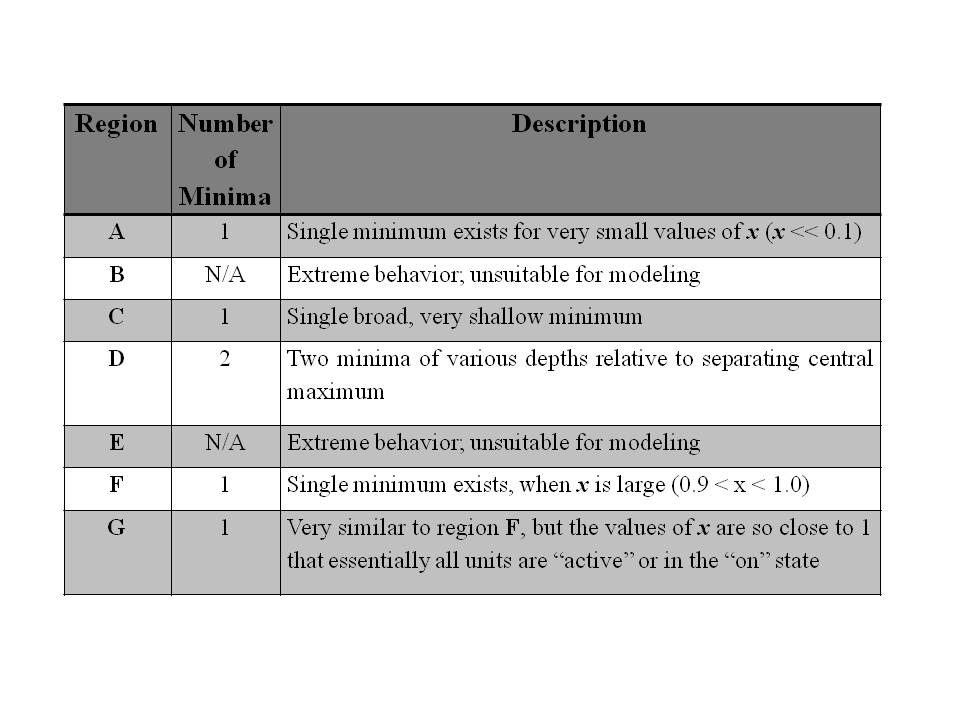
The important thing about this phase space diagram
, and the distinct regions within it, is that it shows how a phase transition could happen between two very different states in a system; one where x is high (most units are in a very active or "on" state x=> 1), and another in which x is low (most units are in an inactive or "off" state, x=>0).

To see this possibility, we examine the case where ε1 is fixed; let's take ε1=3. Then we examine the system for increasing (negative) values of a=ε2/ε1. This means, we trace a vertical line, going from top to bottom, near the center of the diagram, where ε1=3. We will go through three different regions; A, then D, then F/G.

When a=-0.5, we are in Region A. This is a "low x" region; most units are inactive or "off." We increase (the negative value of) a to -1.5, and move to Region D. There are two minima in this region; the system can be either in a low or high value for x. We increase a to -2.5, and move to Region F. There is a single minimum in this region, for x close to 1.

In sum, using the starting equation for free energy given in this post, we have a resulting "phase space" which includes the possibility of both low-value and high-value regions for x satisfying an equilibrium state. There is also a middle region, one in which either a low or high value of x is possible. That means that the phase transition between the low-value and high-value states can be subject to hysteresis; it can be memory-dependent. Often, in practical terms, this means that if the system starts off in a "low-x" state, it will stay in that state until the "free energy minimum" completely disappears, and the system is forced to abruptly shift into a "high-x" state. Similarly, if it is in a "high-x" state, it may stay in that state (while the parameter a continues to change) all the way from Region F through Region D, until the system moves into Region A, and is forced back into a "low-x" state once again.

This equation is used to explain hystersis as well as phase transitions in memory-dependent systems, such as ferromagnets. In this case, a ferromagnetic material that is disordered (different domains are randomly aligned) will become ordered (almost all the domains will align their magnetic fields) when put into an external magnetic field. They will maintain their alignment for a long time. It will take a significant change in external circumstances (e.g., raising the temperature a great deal) to destroy the alignment and bring the ferromagnet back into a disordered state once again. Then, a lot of effort (a significant magnetic field) would be required to re-align the domains.

We know that this equation is good for describing certain physical systems. The question is: to what extent could we apply this to other, more complex systems? And if we did so, would we learn something interesting?

Cloud Computing - and Complex Nonlinear Systems

Cloud Computing Course - Fall, 2010 - George Mason University

A little over a year ago, Jenn, a dear friend and colleague, told me, "Alianna, this work needs to be done on a cloud. And the best way to go is to use the Google App Engine cloud and Python as the programming language."

At that time, I didn't know the first thing about the Google App Engine, Python, or anything else that was cloud-related. But within a few days, I committed to this as the "best way to go," And by the end of the week, I had lined up a commitment to teach Python (as a programming language) and the Google App Engine (as a cloud platform) in a cloud computing class that I would teach at Marymount, in the fall of 2009.

Now, I'll be teaching a greatly upgraded version of this course at George Mason University, in the Applied IT Department, during the fall of 2010 (Wednesdays at 4:30PM, Prince William Campus). Once again, my own cloud computing website will be the "home" for all the goodies - links to the best articles and references, and my entire "programming to the Google App Engine cloud" book-on-the-web.

Today, I'll be listening to Thomas Bittman's (from Gartner) discussion of virtualization to private clouds. He's got a number of YouTube links available - I'll screen them and put the best links on my cloud computing website. See you there!

Returning to the Blog -- and to "Origins ..."

Dear Ones --

A year to the day. Exactly. That's admittedly a long time off between blog postings.

And of course, much has gone on since then. We've started a financial recovery, but the coming commercial mortgage crisis looms. We've endured a winter of record snowfalls, had abnormally high-temperature early April, Tennessee just had record-breaking rains and lost lives to flooding, and we're now in a somewhat more typical and stable weather pattern - meaning progressive fronts and rains, but in a steady and "normal" manner.

And of course, in the past few months, we've had multiple earthquakes, the Iceland volcano (still erupting), and now - contributing man-made environment stress - the oil spill off the Gulf Coast (still gushing).

By themselves, no one particular event - no matter how traumatic - indicates a world-wide crisis or significant shift. It is when we take these as a whole that complex trends emerge. Specifically, we are looking at the possible interactions between events, and event trends.

Interactions that will be highly nonlinear. This means, predicting outcomes will be much more difficult.

We begin with assessing just one contributing factor; earthquakes.

Using data provided by the multiple earthquakes, we don't - on simple visual inspection - see much of a trend increase with data gathered over this past decade.

Some authors present evidence for a significant increase in earthquake frequency; one that goes well beyond the increased world-wide availability of seismograph recording.

Fred Tasker gives a more conservative view, in
Does this mean earthquake frequency is increasing?. He notes, quoting respected geologists, two important points:
(1) Earthquake impacts are a function of not only magnitude, but also the geological substrate in which they occur; e.g., poorly consolidated sedimentary soil fares less well than other types, and
(2) We should not take earthquakes along one fault line as indicative of likely earthquake activity along other major fault lines.

Many volcanoes, like earthquakes, occur on earth's fault lines - the areas where tectonic plates interact.

(More to come ...)

What is interesting here (and perhaps essential to our futures) is that we have the possibility of nonlinear systems evolution. This means that we can't predict what will happen with simple, linear "rate increase" equations.

Look for good reference materials on my website; look for frequent updates!